Click on figures for larger images.

Figure 6. Comparison of the Simulating WAves Nearshore (SWAN) grid G1 and WavewatchIII® model output of significant wave height (A,D,G), peak wave period (B,E,H), and mean wave direction (C,F,I) versus observations at National Data Buoy Center (NDBC) buoys 42040, 42012, and 42007. Operational WavewatchIII® does not archive mean direction, so this variable cannot be assessed. G1 has a spatial resolution of approximately 500 m and encompasses the northern Gulf of Mexico. The spatial extent of the grid and location of the buoys used for model assessment are shown in figure 1. [m, meters; s, seconds; deg, degrees]

Figure 7. Comparison of Simulating WAves Nearshore (SWAN) and WavewatchIII® G2 model output of significant wave height (A,D), peak wave period (B,E), and mean wave direction (C,F) versus observations at National Data Buoy Center (NDBC) buoys 42012 and 42007 for each scenario. Operational WavewatchIII® does not archive mean direction, so this variable cannot be assessed. G2 has a spatial resolution of approximately 300 m and encompasses the western half of the northern Gulf of Mexico. The spatial extent of the grid and location of the buoys used for model assessment are shown in figure 1. [m, meters; deg, degrees]

Figure 8. Time series above shows a portion (January 1, 2011, through March 31, 2011) of the entire probabilistic wave reconstructed time series (August 24, 2000, to January 31, 2013) at buoy 42012 comparing the observations (black), reconstructed values (red; Long and others, 2014), and measurement at offshore buoy 42040 (blue). [m, meters; s, seconds; deg, degrees]

Figure 9. Time series above shows a portion (January 1, 2003, through March 31, 2003) of the entire probabilistic wave reconstructed time series (December 4, 1995, to December 30, 2013) at buoy 42007 comparing the observations (black), constructed values (red; Long and others, 2014), and measurement at offshore buoy 42040 (blue). [m, meters; s, seconds; deg, degrees]

Figure 10. Comparison of wave time series constructed using probabilistic method and observations at National Data Buoy Center (NDBC) buoy 42012 for April 2, 2010, to December 30, 2013 (left column), and comparison of the WavewatchIII® dataset and the observations for the same time period (right column). Comparisons of (A, B) significant wave height, (C, D) peak wave period, and (E) mean wave direction. WavewatchIII® output is every 3 hours, whereas Simulating WAves Nearshore (SWAN) results are hourly, resulting in a larger number of points. [m, meters; s, seconds; deg, degrees]

Figure 11. Comparison of wave time series constructed using probabilistic method and observations at NDBC buoy 42007 for the time period January 19, 2005, to February 15, 2008 (left column), and comparison of the WavewatchIII® dataset and the observations for the same time period (right column). Comparisons of (A, B) significant wave height, (C, D) peak wave period, and (E) mean wave direction. WavewatchIII® output is every 3 hours, whereas Simulating WAves Nearshore (SWAN) results are hourly, resulting in a larger number of points. [m, meters; s, seconds; deg, degrees]

Figure 12. Model sensitivity to wave diffraction in grid G4 with pit 1 present for scenario H6_D7. (A) Significant wave height (in meters) results with diffraction on, (B) Significant wave height results with diffraction off, (On minus Off), difference in significant wave height from both results. [deg, degrees; m, meters]

Figure 13. Model sensitivity to wave triads in grid G4 with pit 1 present for scenario H6_D7. Significant wave height (in meters) results with triads on (A), significant wave height results with triads off (B), difference in significant wave height from both results (On minus Off). [deg, degrees; m, meters]

Figure 14. Weighted average significant wave height for the (A) baseline, no pit bathymetry, (B) bathymetry including borrow pit 1 (change from baseline shown in D), and (C) bathymetry including borrow pit 2 (change from baseline shown in E). Borrow pits are outlined in white. The average is created from the output of individual scenarios, weighted by their percentage occurrence over the time period December 1995 through December 2013 (fig. 2). The pits create a shadowing effect originating from the corners.

Figure 15. For 135 locations (A, black line) along Breton Island (0 m contour shown in green), longshore transport rate (B; eq. 1) for each of the 116 wave scenarios (fig. 2) for the no pit case. Red colors indicate northerly transport and blue colors indicate southerly transport. Moving from left to right in (B), the magnitude of transport increases for larger wave scenarios. Because the dominant wave direction for storms is from the south and southeast (fig. 2), there are few large wave scenarios with predominantly southerly directed transport. [m, meters]

Figure 16. For 135 locations (A, black line) along Breton Island (0 m contour shown in green), change in the longshore transport rate (eq. 1) with the addition of pit 1 (B) and pit 2 (C) for each of the 116 wave scenarios (fig. 2). Red colors indicate a positive change in transport (more northerly or less southerly) and blue colors indicate negative change transport (more southerly or less northerly).

Figure 17. For 135 locations (A, black line) along Breton Island (0 m contour shown in green), average longshore transport rate (B, LSTR) calculated by weighting each of the 116 individual scenario results by its frequency of occurrence in the wave climatology (fig. 2). The change in magnitude of the weighted average longshore transport rate (C) with the addition of the pits is an order of magnitude less than the baseline values, and the overall pattern in transport is the same (B).

Figure 18. Gradient of average longshore transport rate (B, LSTR) constructed from the longshore transport calculated using wave conditions at 135 locations (A, black line) along Breton Island (0 m contour shown in green) for each of the 116 individual scenario results (e.g., fig. 15 for the no pit case) by weighting each scenario by its frequency of occurrence in the wave climatology (fig. 2). The change in magnitude of the gradient of the LSTR (C) with the addition of the pits is an order of magnitude less than the baseline values, and the overall pattern in transport is the same (B). Positive values in (C) indicate more accretion or less erosion, negative values indicate less accretion or more erosion.

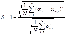
An accurate assessment of the effects of proposed borrow pits on inshore wave climatology relies on the skill of the scenario-based wave modeling approach in predicting the nearshore wave field. A comparison of wave model results to observations at buoys within the model domains for grids G1 and G2 are described in the section “Numerical Model Assessment;” grids G3 and G4 did not encompass buoys to be used for comparison. Included are (1) a comparison of the shallower wave buoy observations to numerical model results, evaluating the ability of the model to represent the spatial transformation of waves, and (2) the accuracy of a scenario-based wave reconstruction for all available buoy times, indicating the ability of the scenario-based approach to capture wave climate at any given time. The results of tests to determine the need to include triad interactions and wave diffraction in the model are described in the section “Sensitivity Analysis.” Finally, analysis of the effects of the proposed wave borrow pit designs on the wave climate around Breton Island is presented in “Effects of Borrow Pits on Nearshore Wave Climate and Longshore Transport.”

Numerical Model Assessment

Data from three NDBC directional wave buoys (42040, 42012, and 42007; fig. 1) were used to assess model output (significant wave height, wave period, and wave direction) for each of the 116 different scenarios for G1 and G2. For G1 (fig. 6), all three buoys were used to compare model outputs for each of the 116 scenarios, whereas for G2 (fig. 7), only buoys 42012 and 42007 were within the bounds of the grid domain. The comparison of wave characteristics to observations at the buoys for the representative times for each scenario assesses the ability of the wave model to propagate waves inshore (for buoys 42012 and 42007) and assesses the accuracy of boundary conditions for buoy 42040. The ability of the G1 and G2 models to predict observations is comparable to the ability of the operational WavewatchIII® model (table 2).

The ability of WavewatchIII® to simulate wave conditions at buoy 42040, which lies just inside the boundary of G1, is acceptable for wave height, period, and direction, illustrating that the WavewatchIII® model resolves wave height conditions sufficiently to provide boundary conditions for SWAN G1 (table 2; fig. 6). The accuracy and precision of WavewatchIII®, however, decreases moving into shallower water, exhibiting higher magnitude bias, much lower values of squared-correlation coefficient (R²), and higher root-mean square error (RMSE). In contrast, the G1 (fig. 6) and G2 (fig. 7) grids retain lower magnitude bias and RMSE and higher values of R² moving into shallower water. The improved predictions are possibly a result of the finer spatial resolution of G1 and G2 (1,500 m and 300 m, respectively, compared to a spatial resolution for WavewatchIII® of ~7.5 km) or better ability of SWAN to resolve shallow water and nearshore wave transformation processes than WavewatchIII®. There is little difference in the RMSE and R² values for buoys 42012 and 42007 in G2 compared to G1 (table 2).

Continuous time series of wave characteristics (height, period, and direction) were constructed at NDBC buoys 42012 (fig. 8) and 42007 (fig. 9) on the basis of probabilistic methods from Long and others (2014). The probabilistic method used offshore buoy observations at NDBC buoy 42040 to identify which of the 116 scenarios was the best match to each time step in the observed record. Time series of wave characteristics were then reconstructed for comparison to observations by extracting G2 model results at the locations of buoys 42012 and 42007 and ordering them on the basis of the sequence of best match scenarios. The accuracy of the time series reconstructions evaluated the ability of the scenario-based approach to capture the full local wave climatology and variability, in addition to the ability of the model to capture spatially variant wave transformation processes within the domain (previously evaluated in the assessment of model accuracy for the representative time steps, as discussed previously). Model assessment included bias, linear regression slope, RMSE, R², and the model skill (S) defined (Gallagher and others, 1998; Reniers and others, 2004) as

(4)

where

A summary of these statistical results is presented in table 3. A value of S = 1 indicates perfect model-data agreement. Model skill is dependent on the ratio between the standard deviation in model-data mismatch and the standard deviation in the data; skill increases when the standard deviation of the data is large compared to the mismatch.

The bias for significant wave height at buoys 42012 and 42007 was low at 3 cm and 5 cm, with an R² of 0.70 and 0.37, respectively (table 3). Model skill, S, was 0.70 and 0.5 for 42012 and 42007, respectively. Bias for peak wave period for both buoys was low (~0.2 s), R² values were lower for peak wave period (~0.2) than for wave height, and the skill score improved (0.73 and 0.67). For mean wave direction, the bias was 3.31 degrees for 42012 and double that (7.67) for 42007, with model skill values similar to peak wave period and somewhat higher R² values (0.58 and 0.55, respectively).

The transformation of waves from the offshore buoy (42040) to the inshore buoys (42012 and 42007) was effectively captured by the reconstruction (figs. 8 and 9). In addition, when winds were blowing from the north, the reconstruction predicted the smaller waves observed at the inshore buoys as a result of short fetch distance between the coastline and the location of observations despite larger measured offshore wave heights. The majority of wave height predictions (height, period, and direction) fall along a 1:1 line with observations (figs. 10 and 11), and accuracy in predicting larger wave heights was improved relative to a previous application of the scenario-based approach by increasing the number of bins for wave heights greater than 2 m (see Long and others, 2014).

The primary concern with the reconstruction application was whether wave characteristics were modeled accurately enough to create robust predictions of alongshore transport. Alternate approaches to predicting nearshore wave conditions are (1) deploying an array of instruments and (2) running a deterministic, time-variant model. Both strategies have the inherent problem of typically capturing a shorter record of time (due to cost or computational expense) than is needed to fully capture the wave climatology; however, comparing the accuracy of the scenario-based model against a deterministic approach is useful for benchmarking it against a commonly used strategy for predicting waves. The model assessment indicates that the probabilistic reconstruction method was able to resolve wave characteristics at least as effectively as the deterministic model Wavewatch III®, while eliminating a bias observed in WavewatchIII® at higher wave periods at buoy 42012. Comparing tables 2 and 3 indicates that the error in wave predictions is similar between the direct simulations (table 2) and the probabilistic reconstruction (table 3). These results indicate that the probabilistic reconstruction used for the assessment is capable of providing results with accuracy similar to assessments that use deterministic model simulations. A previous assessment of the wave climatology approach (Long and others, 2014) also found this approach as accurate as both a Bayesian approach to transforming waves between two locations with historical observations to train the model and a deterministic model run on the same numerical model domain, the latter approach of which is often employed in modeling borrow pit effects on wave climatology (for example, Benedet and List, 2008; Adams and others, 2011).

Back to Top of Page

Sensitivity Analysis

Sensitivity tests were perfomed on grids G3 and G4 to determine the effect of triad wave-wave interactions and wave diffraction on the wave model predictions when a borrow pit was present (pit 1 used for comparisons). Comparison of model scenarios with diffraction turned on versus off in the SWAN model showed minimal change (less than 1 cm) in significant wave height (fig. 12), and thus diffraction was not included in runs analyzing borrow pit impact. Triad wave interactions are relevant to shallow water wave transformation, and sensitivity testing was undertaken to determine triad effects on the G3 and G4 grids. Triads did prove to alter the wave model output enough (~10 cm) (fig. 13) to prompt use of these wave interactions in all of the G3 and G4 modeled scenarios. In particular, wave heights near Breton Island were reduced with the inclusion of triads, possibly as a result of greater dissipation due to bottom friction of the higher frequency (longer period) waves that were generated. Note, one other possible explanation would be that SWAN integration of energy to calculate wave height excluded the higher frequencies generated through triad interactions; however, the version of SWAN used (41.01) integrates over the entire range of user-defined frequencies, which at 0.04–1 Hertz includes the range of frequencies expected to be generated through triads (Herbers and others, 2000).

Impacts of Borrow Pits on Nearshore Wave Climate and Longshore Transport

The effect of the proposed borrow pits on the wave climate around Breton Island was first assessed by calculating a weighted average wave height over the model domain for the baseline (no pit), pit 1, and pit 2 configurations. To compute this composite wave height distribution, the wave height results for each scenario were weighted by the frequency of occurrence from the wave climatology (fig. 2). Comparing the weighted average wave height for the three configurations showed that the wave climate was only noticeably modified in the immediate vicinity of the borrow pit, resulting in a slight shadowing effect originating from the western corners of each pit (fig. 14). The magnitude of the change in weighted average wave height was less than 10 cm, or 5 percent of the baseline wave height, with no discernable change in wave height extending to the nearshore contours around Breton Island. The maximum change in significant wave height for a single scenario was an increase of 74 cm, occurring on the northeast side of borrow pit 1 (fig. 3) for scenario H8_D1 (fig. 2) when the wave conditions in the baseline case at that location were 1.6 m.

The longshore transport rate (LSTR) around Breton Island varied by wave scenario, with the largest transport rates associated with larger offshore wave heights (fig. 15; no pit case). Transport magnitude and direction also varied alongshore with incident wave direction.

The LSTR with the addition of the borrow pits (fig. 16) was similar to the LSTR without the pits, with a change of less than 0.004 cubic meters per second (m³/s) (approximately 10 percent of the magnitude of the baseline condition without borrow pits).

Changes in the transport were also assessed by calculating the alongshore variant average LSTR (fig. 17) weighted by the frequency of occurrence of the 116 wave climatology scenarios (fig. 2). The shape of the alongshore variant LSTR curve did not change with the addition of the borrow pits, and the change in transport magnitude was an order of magnitude less than the baseline case.

Also considered were changes in the gradient of alongshore variant average LSTR (fig. 18). In all cases (pits and no pit), the model predicted accretion at the northern and southern ends and erosion in the center of the island arc. Changes in the gradient of transport were an order of magnitude less than the gradient for the no pit case. The overall shape of the gradient in LSTR did not change with the addition of the pits, and no new convergences or divergences were identified that would potentially be associated with the formation of accretional or erosional “hot spots.” In the case of pit 2 (fig. 1), the magnitude of erosion would be expected to decrease slightly in a region toward the southern end of the island (fig. 17), with slightly more erosion to the north and slightly less accretion to the south of that stretch of island.

Back to Top of Page