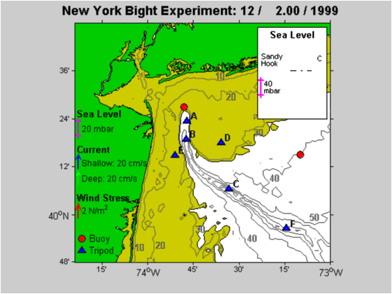
The current, wind stress, and bottom pressure observations collected as part of the Hudson Shelf Valley winter experiment are presented as an animation. All time-series data in the animation were low-pass filtered to remove the tidal motions and to emphasize the wind-driven events. The wind stress and currents are shown as an arrow that originates at the station location and points in the direction of the current flow. The water depth at which waves were sufficiently strong to resuspend sediments was calculated from the Ambrose Tower wave data: areas shallower than this critical depth are shaded brown in the animation. An inset in the upper corner of the animation shows the difference between low-passed sea level at Sandy Hook and bottom pressure at Station C as a proxy for the offshore pressure gradient (Barometric pressure measured at Ambrose Light tower was added to sea level elevation at Sandy Hook to obtain bottom pressure comparable to that measured at Station C). Bottom pressure (minus the mean) is also shown at Sandy Hook and Station C as a pink bar.

The matlab file containing data used to create this animation is included in this data report. The mercator projection was created using Rich Pawlowicz's M_Map toolbox package available at www2.ocgy.ubc.ca/~rich/#M_Map. Individual frames were created as ppm files using programs included on the Matlab m-files page; frames were assembled into the final animation using Videomach software available at www.gromada.com/VideoMach.html.

NOTE: This animation is in .flc format. A reader, such as Quicktime, which can open files of this type is required. Quicktime may be downloaded at www.apple.com/quicktime/download/. For more information on .flc movies, see The FLI/FLC Animation Format (woodshole.er.usgs.gov/operations/modeling/flc.html).