Oceanographic Observations, Hudson Shelf Valley, U.S. Geological Survey Open-File Report 02-217, List of Figures

Identifier symbol and link to USGS Home page

Oceanographic Observations, Hudson Shelf Valley, U.S. Geological Survey Open-File Report 02-217

List of Figures

Non-Data Figures:

PDF Containing All Non-Data Figures [66 MB]

Figure 1	Map showing the location of the Hudson Shelf Valley offshore of New York.
Figure 2A	Schematic of mooring deployed at station A .
Figure 2B	Schematic of mooring deployed at station B.
Figure 2C	Schematic of mooring deployed at station C.
Figure 2D	Schematic of mooring deployed at station D.
Figure 2E	Schematic of mooring deployed at station E.
Figure 2F	Schematic of mooring deployed at station F.
Figure 3	Locations of Conductivity-Temperature-Depth (CTD) stations (black triangles) made December 5-7, 1999 on RV Oceanus.
Figure 4	Locations of Conductivity/Temperature Depth (CTD) stations (black triangles) made April 15, 2000 on RV Endeavor.
Figure 5	A bottom tripod system being deployed from RV Oceanus.
Figure 6A	The stern deck of the RV Oceanus loaded with 3 large tripods (deployed at stations A, B and C) and 1 small tripod (deployed at stations C and D).
Figure 6B	Modular Acoustic Velocity Sensor (MAVS) mounted on small tripod frame.
Figure 7A	The stern deck of the RV Oceanus showing a large bottom tripod, surface buoy, and other mooring gear.
Figure 7B	A micropod being recovered.
Figure 8A	The sensor of the 3 frequency (1, 2.5 and 5 mHz) Acoustic Backscatter System (ABS).
Figure 8B	Lower portion of a Benthic Acoustic Stress Sensor (BASS) tripod system on the deck of the RV Oceanus.
Figure 9	SEACAT with transmissometer and tube sediment trap.
Figure 10	Optical backscatter sensor (OBS) and SeaBird conductivity and temperature sensors attached to the horizontal strut of a tripod frame.
Figure 11	Bracket on bottom of surface buoy used for mounting a MicroCAT to measure near-surface temperature and salinity.
Figure 12	A McLane Labs Water Transfer System (WTS 6-24-47FH) in the laboratory prior to deployment on the tripod at station A.
Figure 13A	Map showing location of instrument mooring, samples for texture analysis, and bottom photographs superimposed on bathymetry and backscatter intensity over shaded relief from multibeam surveys at site A.
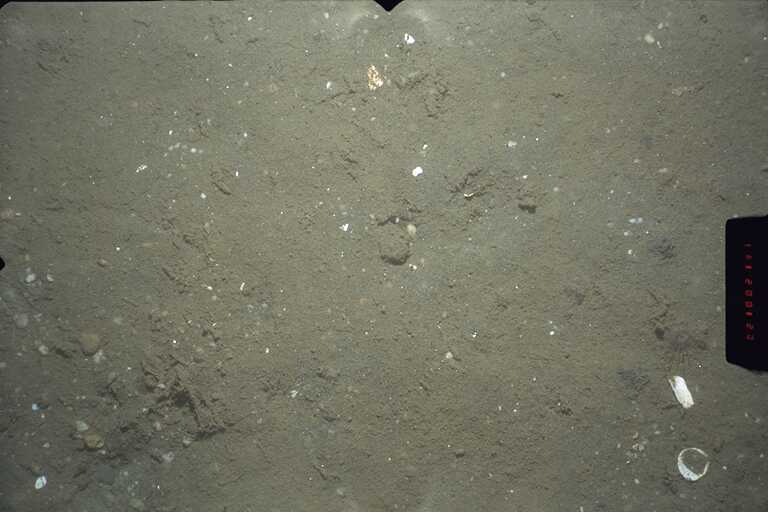
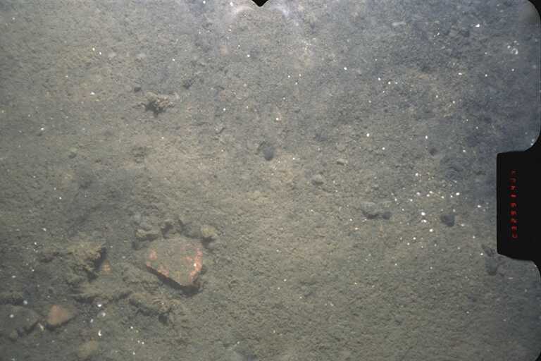
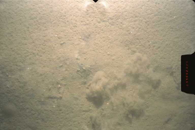
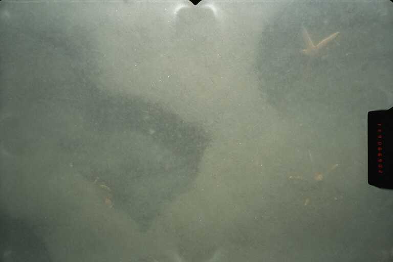
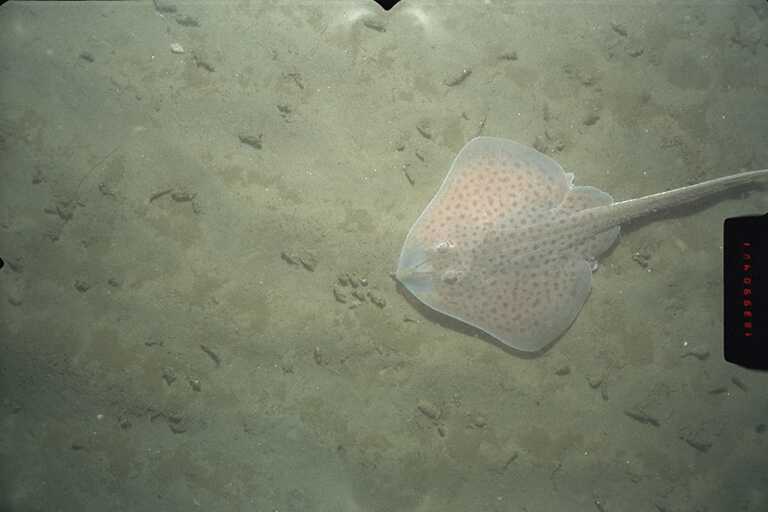
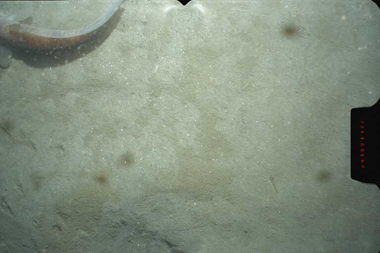
Figure 13B	Bottom photographs at site A, December 1999 (37580021, 21620080). Field of view is nominally 76x51 cm.
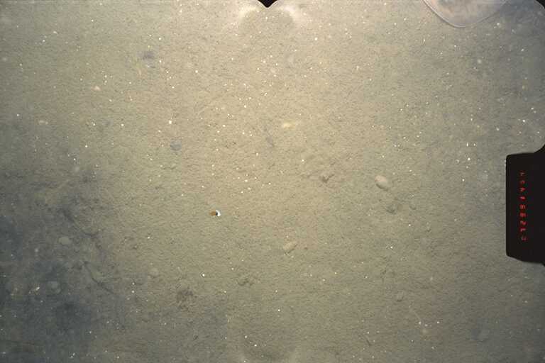
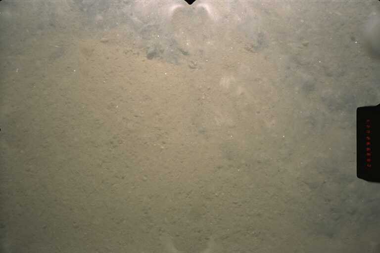
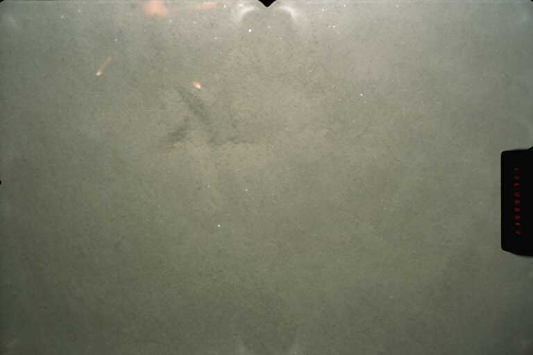
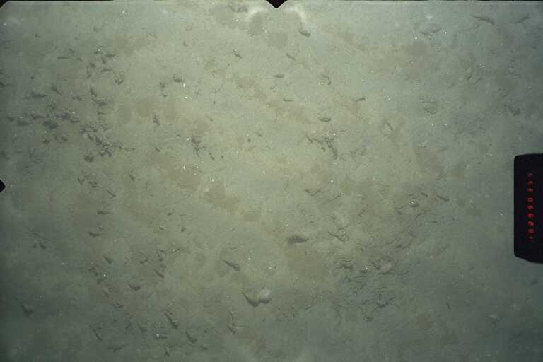
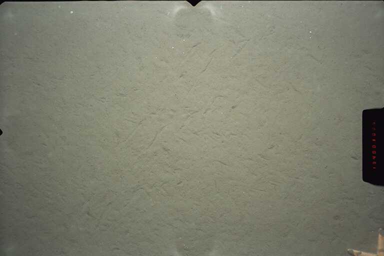
Figure 13C	Bottom photographs at site A, April 2000 (32610054, 32610058, 32610060). Field of view is nominally 76 by 51 cm.
Figure 14A	Map showing location of instrument mooring, samples for texture analysis, and bottom photographs superimposed on bathymetry and backscatter intensity over shaded relief from multibeam surveys at site B.
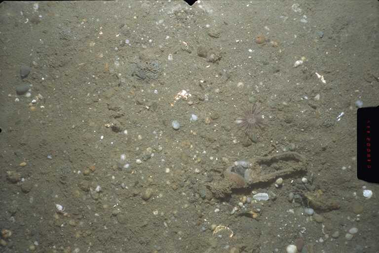
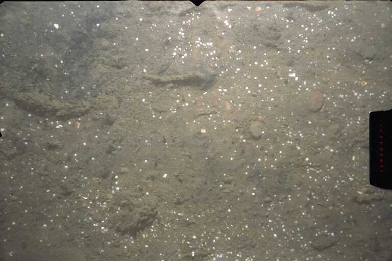
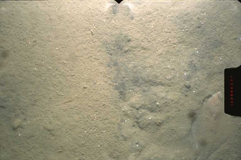
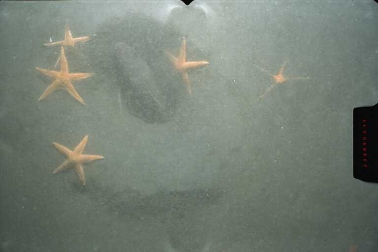
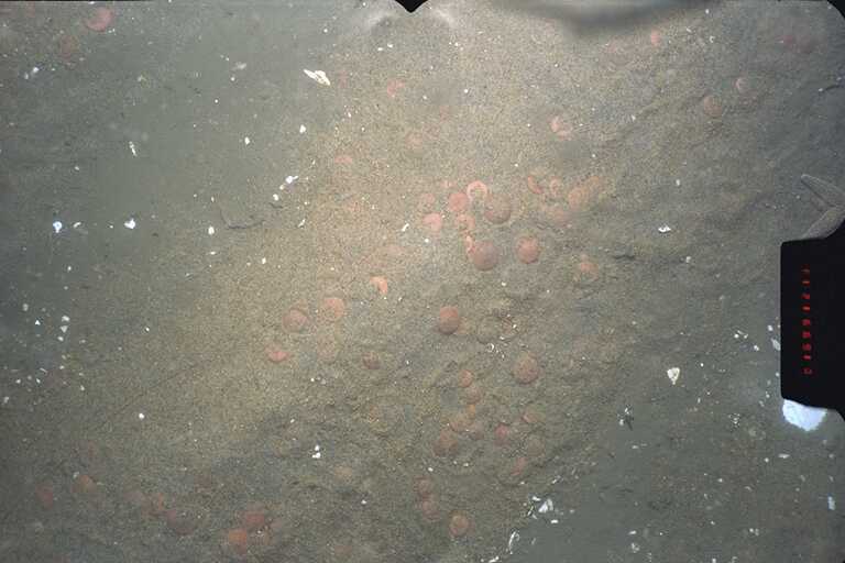
Figure 14B	Bottom photographs at site B, December 1999 (21620075, 21620069, 21620065, 21620062, 21620052 and 21620048). Field of view is nominally 76 by 51 cm.
Figure 15A	Map showing location of instrument mooring, samples for texture analysis, and bottom photographs superimposed on bathymetry and backscatter intensity over shaded relief from multibeam surveys at site C.
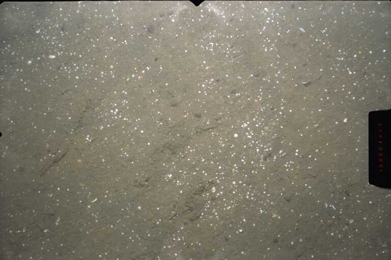
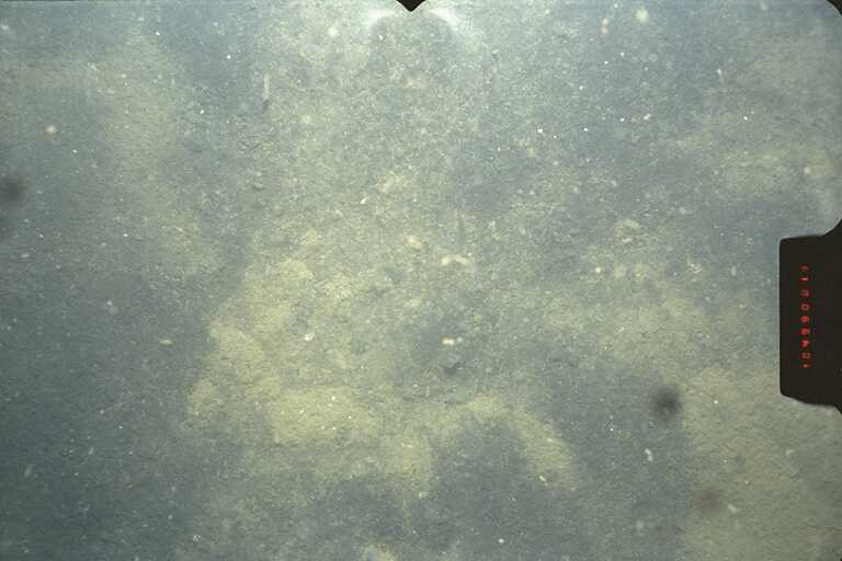
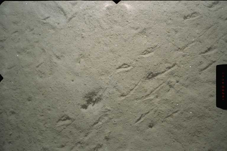
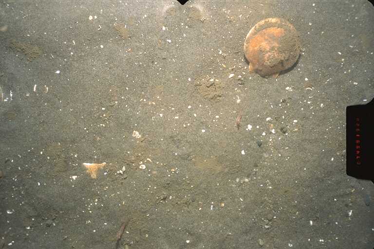
Figure 15B	Bottom photographs at site C, December 1999 (37510047, 37510034, 37510027, 37510020). Field of view is nominally 76 by 51 cm.
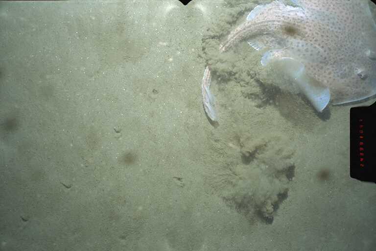
Figure 15C	Bottom photograph at site C, April 2000 (32610043). Field of view is nominally 76 by 51 cm.
Figure 16A	Map showing location of instrument mooring, samples for texture analysis, and bottom photographs superimposed on bathymetry and backscatter intensity over shaded relief from multibeam surveys at site D.
Figure 16B	Bottom photographs at site D, December 1999 (37510070, 37510071). Field of view is nominally 76 by 51 cm.
Figure 16C	Bottom photographs at site D, April 2000 (32740004, 32740005). Field of view is nominally 76 by 51 cm.
Figure 17A	Map showing location of instrument mooring, samples for texture analysis, and bottom photographs superimposed on bathymetry and backscatter intensity over shaded relief from multibeam surveys at site E.
Figure 17B	Bottom photographs at site E, December 1999 (37580037, 37580028, 37580027, 21620078). Field of view is nominally 76 by 51 cm.
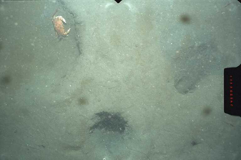
Figure 17C	Bottom photograph at site E, April 2000 (32740019, 32740018, 32740016). Field of view is nominally 76 by 51 cm.
Figure 18A	Map showing location of instrument mooring, samples for texture analysis, and bottom photographs superimposed on bathymetry and backscatter intensity over shaded relief from multibeam surveys at site F.
Figure 18B	Bottom photographs at site F, December 1999 (37510010, 37510007, 37510006). Field of view is nominally 76 by 51 cm.
Figure 18C	Bottom photograph at site F, April 2000 (32610035). Field of view is nominally 76 by 51 cm.

Data Figures:

PDF containing all data figures [44 MB]

HTML location of links to individual data figures:

ATTN, OBS, and ABS	Time series plots of beam attenuation and optical backscatter from each station.
Current (By Station)	Plots of current observations for each station.
Current (All Stations)	Low-passed wind stress and current observations at selected depths from all stations..
Current (Mean and Ellipse)	Plots of low-passed wind stress and monthly mean current flow and variability for each station.
Current Scatter Plots	Scatter plots of eastward and northward current velocity at each station.
Currents (Sorted)	Plots by station of the percentage of current in a particular direction at a particular speed.
Residual Flow	Maps showing mean flow and low-frequency current elliipse at 15 m and near-bottom.
Tidal Ellipses	Maps showing tidal ellipses at 15 m.
Hydrographic Data (Endeavor)	Plots of CTD cast data from the Endeavor cruise: temperature, salinity, sigma t, beam attn., and fluorescence.
Hydrographic Data (Oceanus)	Plots of CTD cast data from the Oceanus cruise: temperature, salinity, sigma t, beam attn ., optical backscatter, and fluorescence.
Meteorological Observations	Time series plot of the meteorological data from the Ambrose Light station.
Meteorological Statistics	Plots comparing meteorological statistics (wind stress, wave height, etc.) from buoys in the vicinity of the study area
Pressure	Time series plots of low-passed wind stress and pressure observations from each station.
Salinity	Time series plots of salinity data from each of the stations.
Statistics	Plots of the monthly statistics of current and temperature for each station.
Temperature	Time series plots of temperature data from each of the stations

To view files in PDF format, download free copy of Adobe Acrobat Reader (www.adobe.com/products/acrobat/alternate.html).

Title Page / Contents / Tables / Figures / Abbreviations / Introduction / Field Program / Observations / Instrumentation / Data Processing / Fouling / Mooring/Data File ID / Results / Digital Data / Acknowledgements / References / Matlab / Supplementary / Metadata

[an error occurred while processing this directive]