Professional Paper 1386–A
Gallery contains 8 columns, so you may need to scroll to the right to see all images.
pp1386a4-fig01 |
pp1386a4-fig02 |
pp1386a4-fig03a |
pp1386a4-fig03b |
pp1386a4-fig04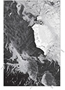 |
pp1386a4-fig05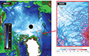 |
pp1386a4-fig06![Figure 6.—Graph of the “Keeling Curve,” the instrumental record of the measurement of the concentration of carbon dioxide (CO2) in the Earth’s atmosphere at the Mauna Loa Observatory, Hawaii from 1958 (313 ppm) to 2009 (390 ppm). From figure at National Oceanic and Atmospheric Administration (NOAA) Web site: [http://www.esh.noaa.gov/gmd/ccgg/trends/co2_data_mlo.html].](images/gallery-4/thumb/pp1386a4-fig06.jpg) |
pp1386a4-fig07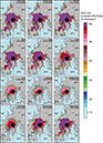 |
pp1386a4-fig08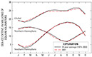 |
pp1386a4-fig09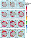 |
pp1386a4-fig10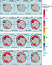 |
pp1386a4-fig11 |
pp1386a4-fig12 |
pp1386a4-fig13 |
pp1386a4-fig14 |
pp1386a4-fig15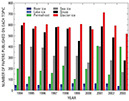 |
pp1386a4-fig16 |
pp1386a4-fig17 |
pp1386a4-fig18 |
pp1386a4-fig19a |
pp1386a4-fig19b |
pp1386a4-fig20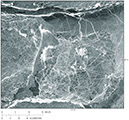 |
pp1386a4-fig21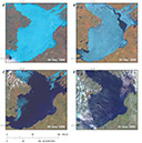 |
pp1386a4-fig22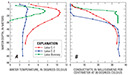 |
pp1386a4-fig23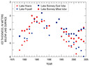 |
pp1386a4-fig24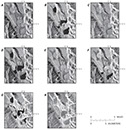 |
pp1386a4-fig25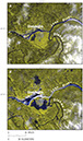 |
pp1386a4-fig26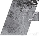 |
pp1386a4-fig27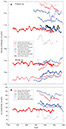 |
pp1386a4-fig28 |
pp1386a4-fig29 |
pp1386a4-fig30 |

![]() U.S. Department of the Interior |
U.S. Geological Survey
U.S. Department of the Interior |
U.S. Geological Survey
URL: http://pubsdata.usgs.gov/pubs/pp/p1386a/gallery-4.html
Page Contact Information: GS Pubs Web Contact
Page Last Modified: Thursday, 01-Dec-2016 16:25:37 EST
