A variety of sensors from several manufacturers were used to measure current, temperature, conductivity, light transmission, and pressure. These sensors were deployed on a variety of platforms (see descriptions below and mooring log), and the data were sampled (see summary of sampling schemes) and recorded by various data logging systems. Seafloor Tripod Systems (figures 13A, 13B, 13C, 13D, 13E, and 13F) USGS seafloor tripod systems provide a platform for long-term deployment of instruments to measure currents and water properties, primarily near the sea floor. At Site A, where measurements included currents 1 mab, temperature, pressure, light transmission, and conductivity within 2 mab, currents throughout the water column, sediment collection rate, and photographs of the seafloor, instruments were deployed on a large tripod frame (figure 13A, 13B). At Site B, where measurements included currents throughout the water column and near-bottom temperature and salinity, instruments were deployed on a smaller frame (figure 13C). For the Massachusetts Bay long-term observations the tripod systems are deployed for about 4 months and data are recorded internally. During the period 1989-2002, two data logging systems were used to obtain the near-bottom observations at Site A. Between 1989 and 1991, a Data Logging Current Meter (DLCM) system was used that measured current with two Savonius rotors and a vane (similar to the VACM current sensor). The DLCM recorded data on a pair of Sea Data tape cassettes or to a hard disk using an Onset Computer Tattletale computer (Butman and Folger, 1979). The DLCM tripod system recorded averages of rotor speed and pressure every 7.5 minutes. Measurements of temperature and conductivity were made at the midpoint of the averaging interval. The instrument also burst-sampled current speed, current direction, and pressure every 2 seconds for 72 seconds (180 seconds if recording on a Tattletale) at the center of each 7.5-minute interval. When the DLCM data were processed, the burst current measurements were vector-averaged to obtain current speed and direction, and the standard deviation of the high-frequency pressure measurements, called PSDEV, was computed as a measure of the bottom pressure fluctuations caused by surface waves. Between 1991 and 2001, near-bottom observations at Site A were made with a MIDAS system that measures current with two BASS (Benthic Acoustic Stress Sensor) 4-axis acoustic current sensors (figure 13D, 13E) mounted nominally at 1.0 and 0.45 mab. Data were recorded using a Tattletale computer (Martini and Strahle, 1992). The MIDAS system recorded pressure and 4 velocity components from each BASS current sensors (Williams, 1985) at 1 hz.. Every 3.75 minutes, MIDAS computed cumulative sums of pressure and current, and recorded them, along with temperature, conductivity, and light transmission measured at the center of the 3.75-minute averaging interval. Average pressure and current were calculated during data processing. BASS current meters are capable of resolving 0.03 cm/s currents; however, this requires a field determination of the zero. Accuracy is affected by the capacitance of the long cables that connect the data logger to the sensors and thus a new calibration must be obtained each time the data logger and sensor wiring is attached to a tripod frame. An accuracy of 0.3 cm/s can be achieved when the offsets generated by these capacitance changes are measured and removed from the data. The BASS current meter voltages were measured when there was no current through the measurement volume, and this 'zero' offset was subtracted from measurements made during the deployment. A set of experiments were performed to determine the most efficient method of calibrating the BASS to 0.3 cm/s accuracy (Morrison and others, 1993). A zero calibration for the BASS current sensors was obtained with the sensors mounted on the tripod system and connected to the MIDAS data logger prior to deployment and after recovery. A water-tight jacket was fitted around the two BASS sensors, filled with water, and data recorded for at least 12 hours to determine an offset under no-flow conditions.

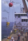
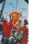
The following figures are in PDF format. Figure 10 Figure 13A Figure 13B Figure 13C Figure 13D Figure 13E Figure 13F Figure 13G Figure 14 Figure 15 Figure 16 Figure 17 Figure 18 Figure 19

The MIDAS system measures conductivity using a Sea-Bird SBE-4 conductivity cell, the same sensors used by Sea-Bird's SEACAT and MicroCAT data loggers described below (figure 13F). On stationary near-bottom platforms such as the tripod, sediment can collect in the conductivity cell and bias the measurement. In the middle 1990's, this was suspected as the cause of a consistent freshening trend over the course of a deployment observed in the bottom tripod conductivity data. Sea-Bird pumps were added to the MIDAS to flush the conductivity cell prior to making a measurement.

Camera

(figure 13G)

A 35-mm Benthos camera system was mounted on the tripod frame approximately 2 m above the bottom (figure 13G) and programmed to take a single photograph of the sea floor every 4 hours. The field of view of the downward-looking camera was approximately 1 m by 1.5 m. The photographs are not included in this data report. See Butman and others 2004a, 2004b, and 2004c for photographs presented as a time-lapse movie.

Acoustic Doppler Current Profiler (ADCP)

(figure 14)

RD Instruments' ADCP's (300 Khz Workhorse) were deployed at Site A (beginning in 1994) and Site B (beginning in 1997) to obtain profiles of currents throughout the water column. The instruments measure currents from the doppler shift of sound reflected from the water column from two pairs of orthogonal acoustic beams (figure 14). The instruments recorded 5-minute averages of current every 15 minutes. To obtain an accuracy of at least 0.4 cm/s for each 5-minute measurement, 300 pings emitted at a rate of 1 ping per second were averaged together. A good primer on the doppler current measurement technique may be found in Gordon (1996). At Site A, the ADCP was initially deployed on a small tripod frame (figure 13C) between 1994 and 1996, then on the large frame beginning in 1996. At Site B, the ADCP was deployed on several versions of a small tripod frame (figure 13C).

Vector-Measuring Current Meter (VMCM)

(figure 15)

Vector-measuring current meters (Weller and Davis, 1980) were used to measure temperature and velocity at a sampling interval of 3.75 minutes ( figure 15). At the long-term station, VMCM's were maintained on subsurface moorings at a depth of 10 mab (nominally 23 m). VMCM's were also suspended from the 40-ft discus buoy, at a depth of 5 m below the surface, from December 1989 until February 1994 when the buoy was discontinued. VMCM's use orthogonal bidirectional propellers and were configured to sample the currents every 0.25 seconds and vector-average internally to calculate averages at the sampling interval of 3.75 minutes. These samples were recorded on 1/4" cassette tapes by Sea Data recorders.

SEACAT

(figure 16)

SEACAT 16 (http://www.seabird.com/) measure conductivity and temperature, and record the voltage signals produced by a transmissometer. SEACAT's were operated with a sampling interval of 3.75 minutes. SEACAT's were attached to the VMCM's that were maintained on subsurface moorings at a depth of 10 mab (nominally 23 m), as well as to the VMCM's that were suspended below from the 40-ft USCG discus buoy, at a depth of 5 m below the surface, from December 1989 until February 1996. Concern that the SEACAT batteries might be disturbing the VMCM compasses caused a change in mooring design in February 1998, with the SEACAT's attached to the moorings immediately above the VMCM at a depth of 11 mab.

MicroCAT

(figure 17)

The MicroCAT was introduced by Sea-Bird as a lower cost, simpler version of the SEACAT 16. The MicroCAT uses the same sensor technology as the SEACAT to collect salinity and temperature data but cannot record data from additional external sensors such as transmissometers. MicroCAT's were used to obtain temperature and salinity measurements where turbidity measurements were not needed. The smaller physical size of the MicroCAT enabled these instruments to be installed on the top floats of the subsurface moorings at Site A and Site B. The recording interval was matched to the other instrumentation, typically every 3.75 minutes.

Transmissometer

(figure 18)

Sea Tech transmissometers measure the transmission of red light (at a wavelength 650 nm) from a Light Emitting Diode (LED) along a 25- cm water path. The voltage output by a photovoltaic detector was recorded by a SEACAT or by a tripod system. Biological fouling of the transmissometer windows often limited the usefulness of the observations. From October 1992 to October 1994, tests of antifouling rings fitted around transmissometer windows showed some reduction in biological fouling (Strahle and others,1994). Antifouling rings have been used on all transmissometers since 1994.

Sediment Traps

Time-series sediment traps (figure 10; figure 19)

A time-series sediment trap (model MK 78HW-13) is manufactured by Mclane Research Laboratories, Inc., East Falmouth, Mass. The function and design of the instrument is described by Honjo and others (1988). It consists of a polyethylene funnel 106 cm long with an 80-cm-diameter mouth. The open end of the funnel is fitted with a honeycomb-shaped baffle made of polycarbonate hexagonal cells 3.2 cm in diameter and 7.5 cm long. Covering the baffle is a polyethylene screen (1 cm mesh). The purpose of the baffle and mesh is to reduce turbulence and resuspension in the funnel and to keep out fish and other organisms that are known to take up residence in open traps. Excluding macrofauna from the trap minimizes their direct contribution of excretion products to the sample.

The funnel directs falling particulate matter into one of thirteen 500-ml plastic bottles which are threaded into a rotating plate under the funnel. Each bottle is advanced to the sampling position under the funnel on a selectable schedule assigned using an internal Tattleatale 8 computer. The sampling interval for each bottle is typically about 10 days for a 4-month deployment. Samples are sealed except for the period they are under the funnel. To reduce the decomposition of organic matter in the period between collection and analysis, each bottle is filled with a solution of 5% sodium azide (NaN₃) in filtered seawater before deployment. The higher salinity (and density) of the azide solution compared to ambient seawater significantly reduces its diffusion out of the trap during the 4-month collection period.

Although this trap was originally designed for long deployments in the open ocean, the size of the funnel mouth and the bottle volume are appropriate for 4-month deployments at 4.5 m above bottom in this coastal setting (water depth 30 m). Typically, there is a measurable amount of sediment in each bottle, even during quiet periods in summer when resuspension events are infrequent. Occasionally, during an unusually strong storm, the magnitude of sediment resuspension is so great that a sampling bottle overfills and sediments accumulate in and plug the throat of the funnel. Under these conditions the remaining bottles are empty when the trap is recovered. A digital image of the bottles from each deployment was taken in order to visually show the changes in collection rate during the deployment period. This information is not included in this report but is available on request.

Traps made simply from standard core tubing were also used on the USGS moorings in order to provide samples at multiple levels in the water column. These traps consist of 60-cm-long polybutyrate tube with a 6.6-cm internal diameter and a wall thickness of 3.2 mm. The bottom of the tube was sealed with a securely taped plastic cap. Baffles consisted of an aramid fiber/phenolic resin honeycomb (trade name: Hexcell) with a cell diameter of 1 cm and a length of 7.5 cm. The material showed no apparent deterioration during exposure to seawater, although it is subject to biofouling. The tube traps are inexpensive to construct and are easily attached to other instruments or to the mooring wire with black electrical tape.

To accommodate different chemical analyses of the trap samples, different preservative solutions were used with little impact on the collection rate. Most traps were filled to within 7.5 cm of the top with a filtered solution of 5% sodium azide in seawater. Some traps at the same location and depth had no preservative, and others were filled with a filtered solution of seawater, 2% buffered formalin with an additional 35 g/kg NaCl. The average standard deviation of trapping rate for the three conditions (azide, formalin, and no poison) was 5% of the mean value. This indicates that the different density gradients in the traps below the Hexcell baffle had little effect on the trapping dynamics of the tube traps.

Trapping efficiency is a factor that must be considered if the results from the tube traps and the time-series traps are compared. A number of studies have discussed the dependence of aspect ratio (height/width), shape, tilt, Reynolds number (UD/k, where U = horizontal fluid velocity, D = trap diameter, and k = kinematic fluid viscosity) and other factors (Butman, 1986; Gardner, 1980, 1986). In this study, a comparison of relative trap efficiency has been determined during a number of field experiments by simply comparing the collection rates in the time-series traps with tube traps fixed at the same location and depth. A summary of the data since 1989 indicates that time-series traps collect at a rate lower than tube traps by a factor of 0.28 +/-0.11. This difference is consistent with a comparison of efficiency between tube traps and funnels up to 50 cm in diameter conducted on the edge of the continental shelf (Bothner and others, 1988).