U.S. Geological Survey Open-File Report 2011-1127
Construction of a 3-Arcsecond Digital Elevation Model for the Gulf of Maine
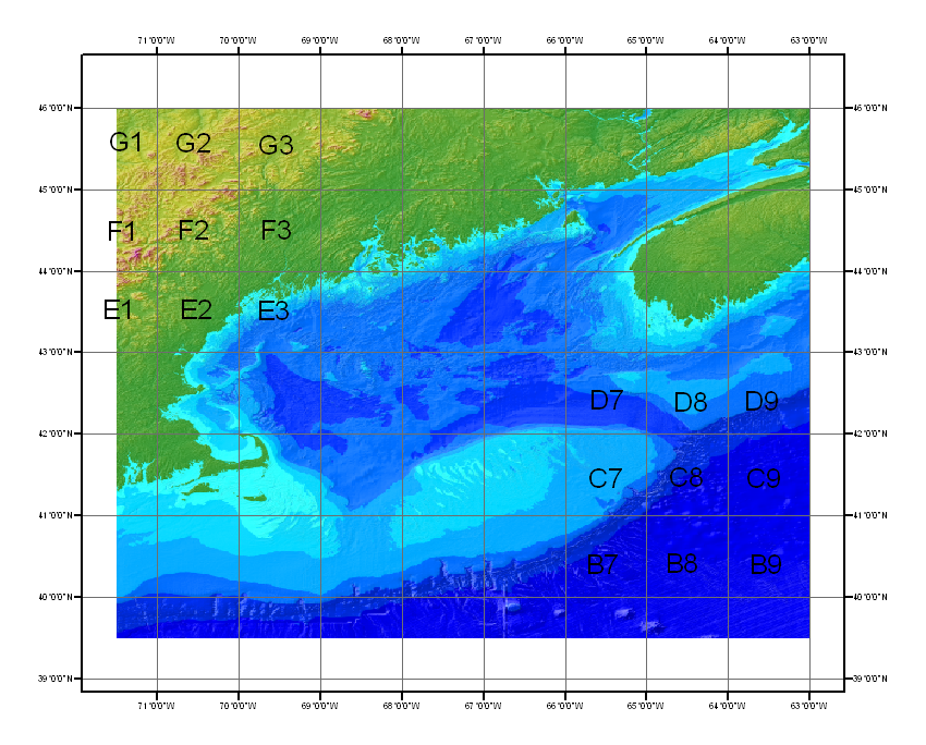
The subregions formed a 7 × 9 array, which for convenience we labeled with rows A through G and columns 1 through 9 (table 1). Table 1. Coordinates of the 1°12' × 1°12' subregions used to generate the 3-arcsecond digital elevation model for the Gulf of Maine. [Latitudes and longitudes are listed in decimal degrees]
The next step was to run the filtered working sub-regions through the GMT surface algorithm. Surface is an adjustable-tension continuous curvature surface gridding algorithm that works by reading (x,y,z) triplets of data from standard input [or xyzfile] and producing a binary grid file of gridded values z(x,y) by solving:
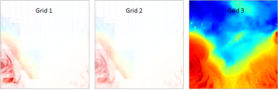
When T = 0, equation 1 gives the "minimum curvature" solution. Minimum curvature can cause undesired oscillations and false local maxima or minima; using T > 0 can be used to minimize the effects of oscillations on minimum curvature. Experience suggests that a value of T approximately 0.25 usually closely approximates the average data points for potential field data, and T should be larger (T approximately 0.35) for steep topography data. T = 1 gives a harmonic surface; no maxima or minima are possible except at control data points (Smith and Wessel, 1990). The construction of the grid for the DEM of the Gulf of Maine used a tension factor of 0.35. This value was chosen because it had less of a "tent-pole"-like effect on the final surface. In addition to the tension option, other options were also used to create the grid. The aspect ratio was set to 0.75 because the gridding process took place using decimal degrees, not projected units, such as meters. The value of 0.75 represents an average value of the anisotropy between latitude and longitude over this domain. The convergence limit was set to 0.1, meaning that the iterative gridding process was deemed to reach convergence when the grid at all cells had stopped changing by more than 0.1 m. Figure 17 shows a comparison of three grids from working sub-region C3. Grid 1 was created with unfiltered data using the GMT xyz2grd command. Grid 2 was created with data filtered by blockmedian and then run through xyz2grd. Grid 3 was created using data filtered by blockmedian and run through the adjustable-tension continuous curvature surface gridding algorithm 'surface'.
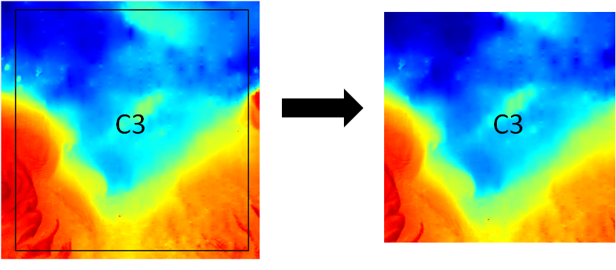
Grid 1 contains all of the raw, pre-processed data at varying resolution. After the data pass through "blockmedian" (grid 2), a single value represents each 3-arcsecond grid cell, with gaps where no data were present within the grid cell. After the data pass through surface (grid 3), a continuous, gap-free grid is obtained. The continuous grid of each subregion was then clipped to 1° × 1° squares using the GMT grdcut tool.
The final cut grid area comprised seven rows of latitude and nine columns of longitude. The new subregions are defined in table 2. Table 2. Coordinates of the final cut grid subregions used to generate the 3-arcsecond digital elevation model for the Gulf of Maine. [Latitudes and longitudes are listed in decimal degrees]
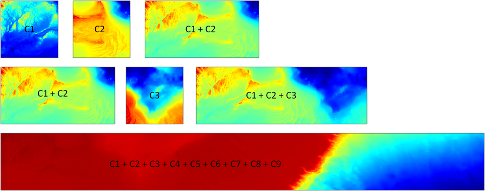
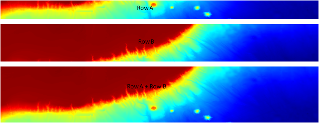
The final digital bathymetry grid was assembled by "pasting" the sub-regions together on a common edge. This was done using the GMT grdpaste command where the user specifies two input grids and a single output grid file name. Grdpaste searches for the common edge and pastes the two grids together to form the final grid. Since there were many subregions of the Gulf of Maine, a pasting method had to be followed. Subregions 1 and 2 of a specific row were pasted together as the base grid. Grdpaste was then run iteratively along each row, pasting the westernmost subregion to the adjacent subregion to the east until each row was complete (fig. 19). Grdpaste was then run for the assembled rows using the same method, working from the southernmost row adding adjacent rows to the north (fig. 20).

| |||||||||||||||||||||||||||||||||||||||||||||||||||||||||||||||||||||||||||||||||||||||||||||||||||||||||||||||||||||||||||||||||||||||||||||||||